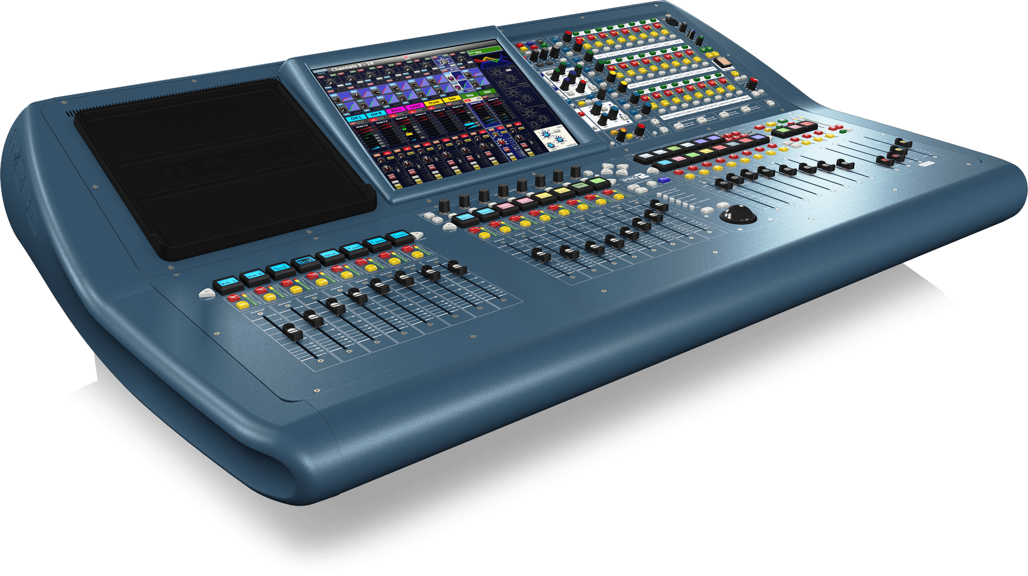
Analog audio mixer designed and assembled in my Circuit Theory class at UW (EE 233)
Abstract:
The purpose of this lab was to combine the knowledge we gained from all of the circuits we experimented with throughout the quarter, including summing amplifiers, voltage followers, filters, and microphone circuits to build a fully-functioning audio mixer. To reach desired passbands and cutoff frequencies, we needed to design the circuit components on our own, and our theoretical findings aligned with those observed in our experimental determinations.
Introduction:
The primary objective of this lab was to design filters according to a given circuit topology and frequency specifications and to incorporate these designs into an audio mixing console. Three filters were designed in this lab by selecting capacitor values to produce desired frequency passbands for each filter. These filters were arranged within an equalizer circuit, which allows gain control over three separate passbands of frequencies. The individual channels passed into the equalizer are then recombined via a summing amplifier and sent to a speaker. The filters designed for the equalizer are brought together with the circuits we have developed over the course of the quarter, including summing amplifiers, preamplifiers, and voltage followers (buffers), to serve their respective functions within the complete audio mixer.
Lab Materials
The components used in this lab were: 6 2.4kΩ, 6 240kΩ, 1 1kΩ and 1 47kΩ resistors. 1 50kΩ rated potentiometer (54), 11 100kΩ rated potentiometers (104), 6 LM348N op-amps. 2 560pF, 2 47 pF (47J), 1 220pF (221), 1 1µF (104), 1 22 pF (220), 1 0.0022µF (222), 1 0.022µF (223), and 1 0.0056µF (562) capacitors. The other lab tools we used to perform the experiment included: a function generator to supply a sinusoidal input, a DC power supply, an oscilloscope to measure the output, a breadboard to build the circuit, and a spectrum analyzer to measure the gain of the circuit. The number of wires required for this lab is very high as there were many connections necessary. On our opamp for the equalizer, we built the buffer and the 3 filters using all the appropriate ports.
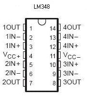
Each op-amp needed a DC power source, and based on the pin-out diagram, we used the 4 and 11 ports to supply our Vcc and Vee of 12 V, respectively. Channel 1 on our oscilloscope displayed our input, while Channel 2 displayed our output wave. The measure function on the oscilloscope was used to experiment and observe which equalizers affected the output gain. We also used autoset and measure functions on the oscilloscope while performing AC sweeps to analyze the frequency-gain behavior of the circuit. The function generator was used throughout the experiment, with variations being made to the magnitude and frequency of our output, the resistance attached to our frequency generator was set to high Z in order to avoid potential problems that could have occurred during the experiment.
Experimental Procedure and Analysis
4.1 Band-pass and Band-stop Filters
We first started by building the band-pass, band-stop filter circuit. We connected our input from our function generator to a node that had two resistors connected, a 240 kΩ resistor and a 2.4 kΩ resistor. The 240 kΩ resistor was connected to the negative input node of the op-amp. The 2.4 kΩ resistor was led into a node on one side of a capacitor (C1) which was connected to both the inputs of a 100 kΩ potentiometer. The output of the potentiometer led into another capacitor (C2) which was connected to the negative input node of the op amp. Another 2.4 kΩ resistor was connected to the node on the other end of the C1 capacitor. From there it was connected to a node that had another 240 kΩ resistor, this 240 kΩ resistor was connected to the negative input node on our op-amp. At the joint connection of the lone 240 kΩand 2.4 kΩ resistors, a connection was then made to the output terminal of our op-amp. The positive input terminal of our op-amp was grounded. The C1 and C2 values were then picked to be 0.0022 µFand 0.022 µFrespectively so our filter could have a center of 1 kHz.
Question 1: What are the resistors and capacitors that you used in this filter?
To obtain the desired center frequency of 1 kHz, we used C1=0.0022 µF, C2=0.022µF, R3=R4=2.4 kΩ, R1=R2=240 kΩ, R5=100 kΩ
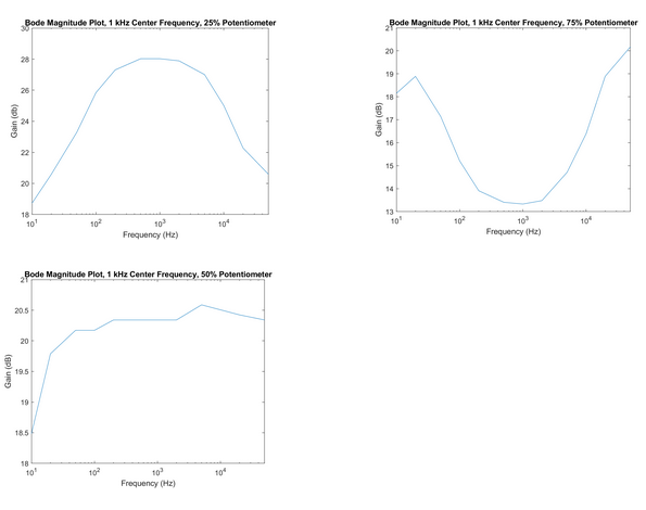
We set up three 100 kΩ potentiometers to have 25 kΩ, 50 kΩ, and 75 kΩ resistances and did the following to get the bode magnitude plots for each specific pot value.
To get the magnitude bode plots of the circuit, we incremented on a basis of 1-2-5 from 10 Hz to 50 kHz, while recording the amplitudes of our input and output peak to peak voltages using the measuring function on the oscilloscope. We then found the gain at each hertz value by taking a ratio of our output voltage over the input voltage. We then converted it to decibels by taking the log base ten of our ratio and multiplying it by 20. A log plot of our data, with the y-axis being the gain in dB and the x-axis being Hz, was made using Matlab.
Question 2: Turn in the hard copy of the gain with your lab report. Use a table to store the center frequency, 3-dB frequencies, and maximum gain for the filter by setting the potentiometers to 25%, 50% and 75%.
1 kHz Center Frequency Adjustable Filter:
Potentiometer Setting
| Center Frequency (Hz)
| 3-dB Frequencies (Hz)
| Maximum Gain (dB)
|
|---|
25% | 1000 | 80, 10000 | 28.0 |
50% | 1000 | n/a* | 20.6 |
75% | 1000 | 100, 10000 | 20.2 |
*Frequencies outside the scope of the measured range
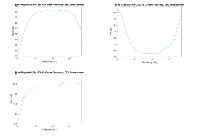
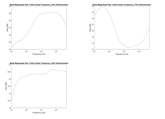
The process to generate bode magnitude plots of our circuit was done again for two new filters, one designed with C1=560 pF and C2=1µF for a filter with a center frequency of 250 Hz, and another designed with C1 = 560 pF and C2 = 0.00560µF for a filter with a center frequency of 4 kHz.
Question 3: What are the resistors and capacitors that you used in these filters? Turn in the hard copy of the gain with your lab report. Use a table to store the center frequency, 3-dB frequencies, and maximum gain for the filter by setting the potentiometers to 25%, 50% and 75%.
To obtain the desired center frequency of 250 Hz, we used C1 = 560 pF, C2 = 1µF, R3 = R4 = 2.4 kΩ, R1 = R2 = 240 kΩ, R5 = 100 kΩ
To obtain the desired center frequency of 4 kHz, we used C1 = 560 pF, C2 = 0.00560µF, R3 = R4 = 2.4 kΩ, R1 = R2 = 240 kΩ, R5 = 100 kΩ
250 Hz Center Frequency Adjustable Filter:
Potentiometer Setting | Center Frequency (Hz) | 3-dB Frequencies (Hz) | Maximum Gain (dB) |
|---|
25% | 800 | 30, 30000 | 28.3 |
50% | n/a* | n/a* | 20.6 |
75% | 800 | 20, 30000 | 16.8 |
*Frequencies outside the scope of the measured range
Despite using capacitor values we determined in the prelab to produce a 250 Hz center frequency, we note that the above Bode plots appear to show a noticeably higher experimental center frequency. The apparent center frequency is somewhere in the range of 600-1000 Hz.
4 kHz Center Frequency Adjustable Filter:
Potentiometer Setting | Center Frequency (Hz) | 3-dB Frequencies (Hz) | Maximum Gain (dB) |
|---|
25% | 4000 | 300, 50000 | 28.3 |
50% | 4000 | n/a* | 20.7 |
75% | 4000 | 300, 30000 | 19.8 |
4.2 Audio Mixer
In this section an audio mixer was designed. Three inputs were taken into a summing amplifier, with one input being a microphone circuit that ran through a pre-amplifier. The summing amplifier was then run into an equalizer circuit which was composed of a buffer op amp circuit that ran into three separate filters. These equalizer filters were of the three we designed in the first part of our lab procedure. The output of the three filters were then summed back up into another summing amplifier. The various amplifiers used in this lab were made using whatever parts we had available to us via the lab kit, and were designed based on amplifiers we made in past labs.
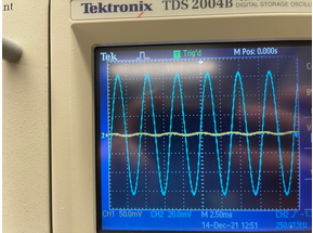
Question 4: Display the input and output waveforms in 2-3 complete cycles on the scope and turn in the hard copy with your lab report.
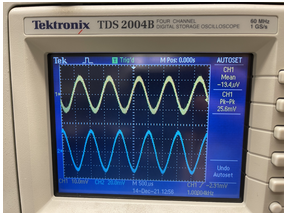
With a sine wave of Vpk-pk=100mVand =250 Hz, our output wave looked like this (blue) :
Figure 1. Output (blue) w/ 250 Hz frequency and 100 mV inputs (yellow)
With the initial sinusoidal input of 100 mV peak to peak voltage with 250 Hz frequency, we adjusted the various potentiometers in our equalizer to see what effects it would have on our output. This process was repeated for inputs with attached frequencies of 1 kHz and 4 kHz.
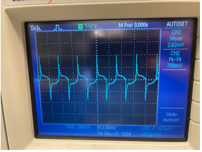
Question 5: Which filter controls the amplitude of the output filter? Turn in hard copies of the scope to support your conclusion.
Each filter exhibited varying degrees of control over the output filter given a 250 Hz sine wave input. When the potentiometer for each filter was adjusted, and the resistance decreased, the amplitude of the output wave greatly increased. This runs contrary to our expectations about the circuit’s behavior, as we would anticipate that only the 250 Hz center frequency passband filter would control the output filter at this frequency. However, we attribute this discrepancy to overlap in the passbands for each filter. That is, given the components used to design our filters, each filter appears to produce high gain at certain shared ranges of frequencies. Thus, we do not observe clear-cut control over the output filter from any one filter at the given frequency.
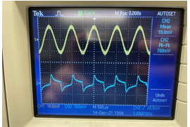
The oscilloscope image below shows the result of adjusting the 250 Hz passband filter given a 250 Hz sine wave input. The resulting waveform resembles those produced by adjusting the 1 kHz and 4 kHz passband filters.
Figure 2. Output (blue) w/ 250 Hz frequency and 100 mV inputs, after adjusting potentiometer for 250 Hz passband filter
Question 6: Which filter controls the amplitude of the output filter at 1 kHz and 4 kHz? Turn in hard copies of the scope to support your conclusion.
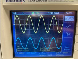
As was the case for the 250 Hz sine wave input, we observed that adjusting each filter given a 1 kHz sinusoidal input resulted in a change in the amplitude of the output. We can see below that adjusting the potentiometer for the 1 kHz center frequency filter produced a change in the output amplitude. Adjusting the 250 Hz and 4 kHz passband filters allowed similar levels of control, however. Again, we attribute this to overlap in the passband frequencies of each filter.
Figure 3. Output (blue) w/ 1 kHz frequency and 100 mV input
Figure 4. Output (blue) w/ 1 kHz frequency and 100 mV inputs, after adjusting potentiometer for 1 kHz passband filter
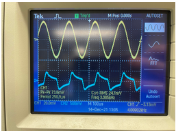
Next, we changed the frequency of the sinusoidal input to 4 kHz and produced outputs on the scope as seen below. Based on the magnitude change of the amplitude, we observed that the filter associated with the 4 kHz cutoff frequency made the greatest impact on the gain of our input. Again, however, the other filters in the equalizer also allowed control over the output filter, presumably for the same reasons discussed above.
Figure 5. Output (blue) w/ 4 kHz frequency and 100 mV input (yellow)
Figure 6. Output (blue) w/ 4 kHz frequency and 100 mV inputs (yellow), after adjusting potentiometer for 4 kHz passband filter
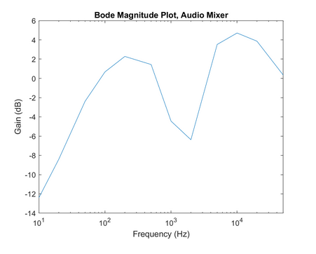
To get the magnitude bode plot of the audio mixer, we incremented on a basis of 1-2-5 from 10 Hz to 50 kHz, while recording the amplitudes of our input and output peak to peak voltages using the measuring function on the oscilloscope. We then found the gain at each hertz value by taking a ratio of our output voltage over our input voltage. We then converted it to decibels by taking the log base ten of our ratio and multiplying it by 20. A log plot of our data, with the y-axis being the gain in dB and the x-axis being Hz, was made using Matlab.
Question 7: Turn in the plot of the gain in your lab report and comment on how many bands you see in the plot.
Observing the plot for our gain in the audio mixer with each potentiometer adjusted to 100%, we see two visible bands.
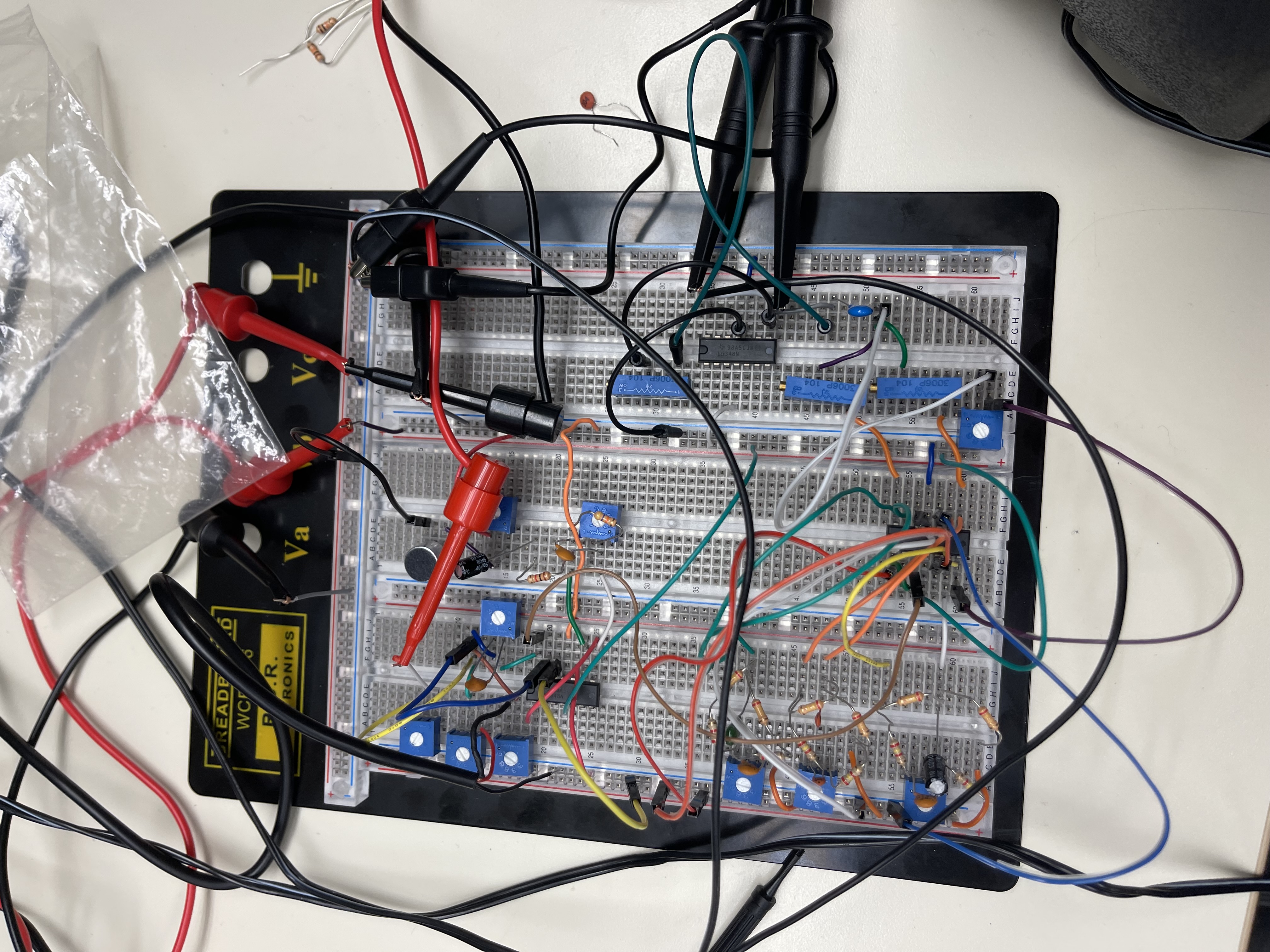
The final product looks something like this:
Completely assembled and functional audio mixer
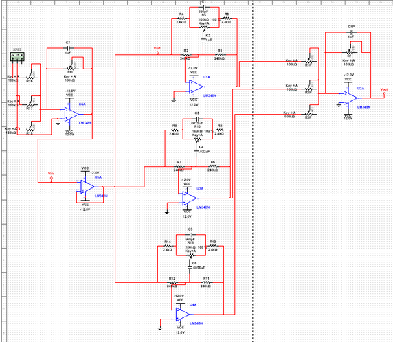
4.3 Simulation in Spice
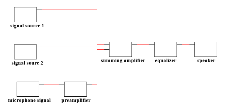
Figure 7. Entire audio mixer circuit schematic in SPICE (excluding pre-amp and microphone)
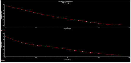
Figure 8. AC Sweep of the output of audio mixer circuit in SPICE with one sinusoidal input (w =1000 kHzVin, pk-pk=1 V
Question E: What does the transfer function look like with only one input track? Describe the roles of each part in the system.
With only one input track, based on the observation from the simulation, the transfer function resembles a non-ideal low pass filter. The system for the audio mixer consists of seven blocks. A microphone, preamp, 2 signal inputs, a summing amplifier, an equalizer, and a speaker/output console. The microphone essentially behaves as an input signal, and the pre-amp is there to balance the input signal or remove the DC voltage offset. The three signal inputs go into a single summing amplifier, which then sums the signals and outputs them into a buffer (voltage follower), which then inputs the signal into three filters, each one corresponding to a different center frequency (250 Hz, 1 kHz, 4 kHz). These three signals are then put through a summing amplifier and then outputted.
Conclusion
Several conclusions were made based on our observations and analysis of the behavior of a bandpass/bandstop filter and a fully functional audio mixer circuit. One of the first important conclusions we reached while performing the procedure with the filter circuit, was that adjusting the potentiometer from a 25% resistance to a 75% resistance altered the behavior of the transfer function of the circuit, changing the circuit from having the behavior of a band-pass filter to performing like a band-reject filter. The next procedure of the lab involved assembling a fully functional audio mixer circuit, which included an equalizer block that required utilizing three filters with the different center frequencies stated above. With the audio mixer circuit, we observed that adjusting the potentiometers associated with each respective center frequency impacted the gain more significantly than the other two filters. Essentially, if the input frequency was equal to the center frequency of a particular filter, the resistance was minimized, and the gain increased. One significant issue we encountered while building the audio mixer was dead spots in our breadboard, which at times prevented us from getting a proper reading on the oscilloscope. If we were to repeat this lab again with the goal of getting the most ideal results, we would use a breadboard that is completely functional and new op-amps to ensure that they are not damaged or not fully functional.
Appendix:
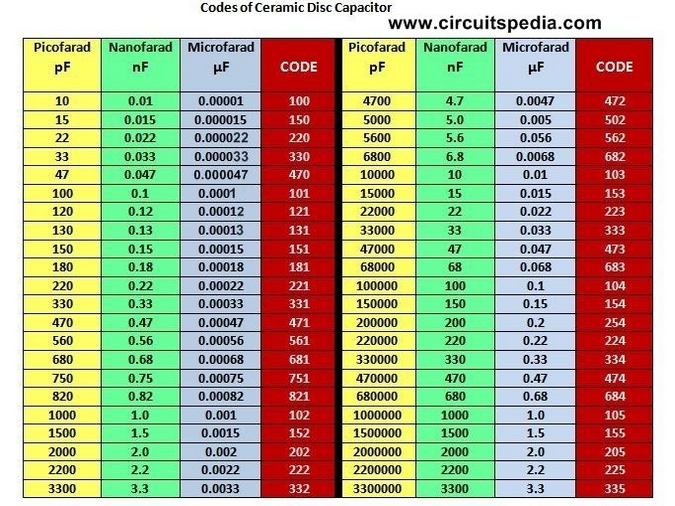
Datasheet used as a reference to find proper capacitor values