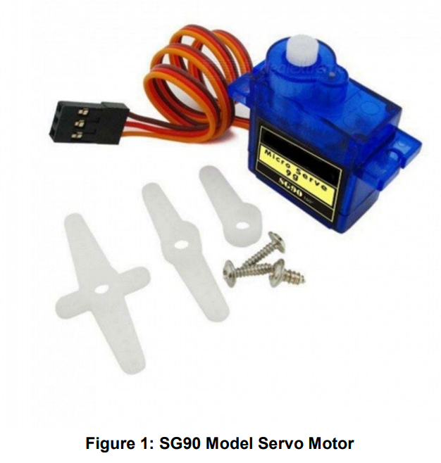
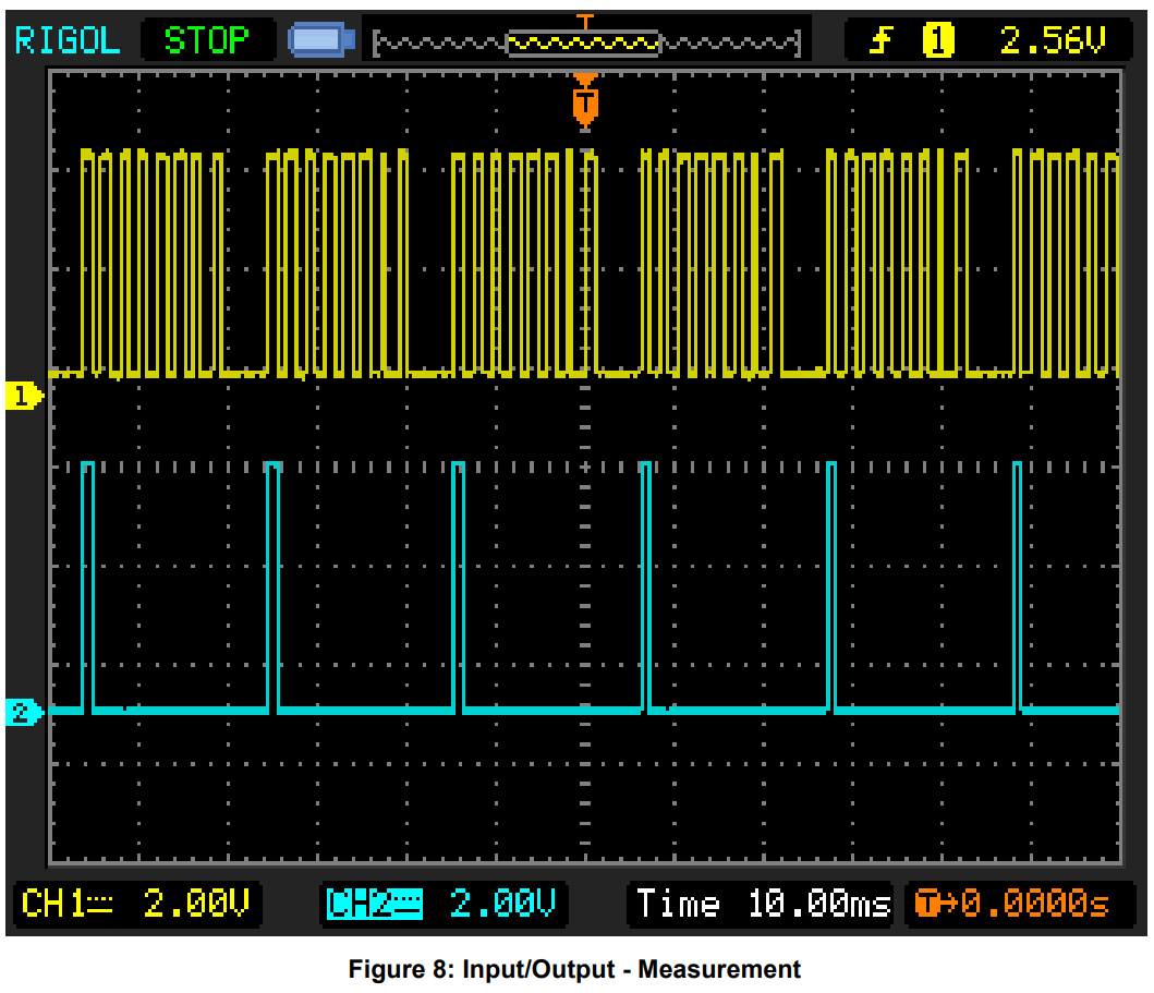
Servo Motors are widely used for commercial and industrial applications as linear or rotary actuators. In this example the SG90 model is used, which is low cost, consumes little power, and is lightweight. This makes these type of servos ideal for consumer device RC toys such as RF-controlled race cars, airplanes, and others.
However, to properly control a servo motor, the electronic driver must generate appropriate voltage patterns to the servo motor DATA pin. The waveforms should be pulses shorter than 2 milliseconds, repeating every 20 milliseconds for one servo motor.
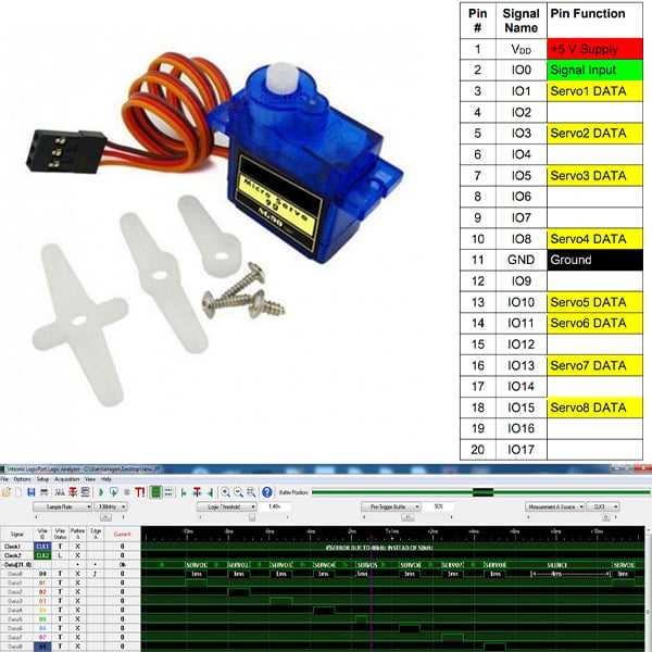
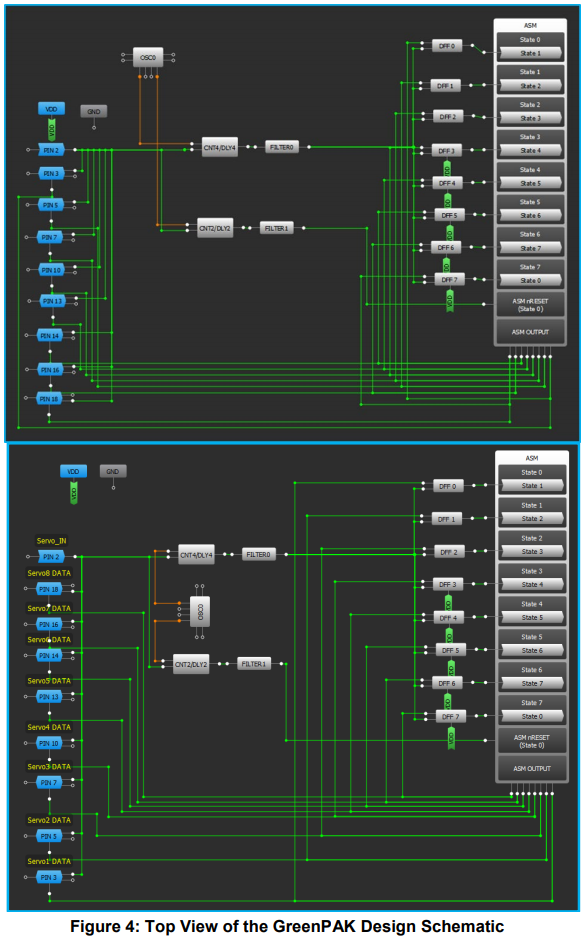
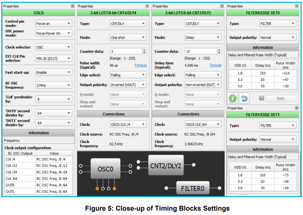
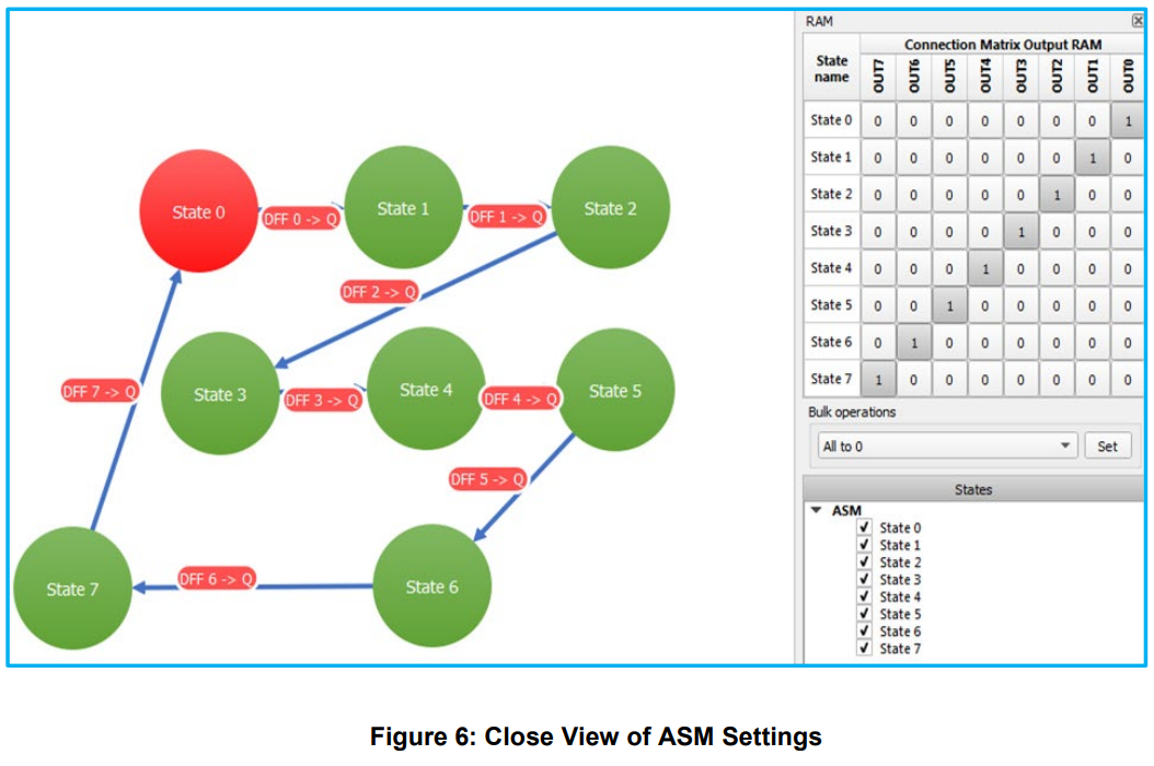
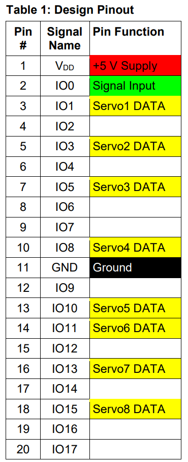
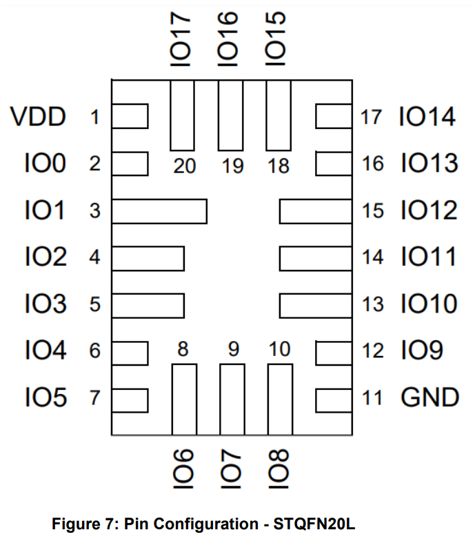
This project will present the design of one 1 to 8 servo motor signal demultiplexer with the SLG46537V GreenPAK™ IC. The designed signal demultiplexer would drive up to 8 servo motors on 8 output pins with the multiplexed signal coming in on 1 input pin. The SLG46537V can also integrate additional functionality, such as additional logic or voltage monitoring, depending upon the system requirements.
The following sections will show:
- A servo motor 1 RF channel signal multiplex;
- The SLG46537V GreenPAK servo demultiplexer design in detail;
- How to drive 8 servo motors with 1 GreenPAK device.
#servoMUX.py###################################################################BEGIN#
import wave
import numpy as np
import matplotlib.pyplot as plt
def repeat48x(series):
return np.concatenate(( series, series, series, series, series, series, series, series, series, series, series, series, series, series, series, series, series, series, series, series, series, series, series, series, series, series, series, series, series, series, series, series, series, series, series, series, series, series, series, series, series, series, series, series, series, series, series, series), axis=None)
silence=-np.ones(200)
pulse10=np.concatenate((np.ones(50), -np.ones(50)), axis=None)
plt.plot(pulse10)
plt.ylabel('pulse 1.0ms')
plt.show()
pulse05=np.concatenate((np.ones(25), -np.ones(75)), axis=None)
plt.plot(pulse05)
plt.ylabel('pulse 0.5ms')
plt.show()
pulse15=np.concatenate((np.ones(75), -np.ones(25)), axis=None)
plt.plot(pulse15)
plt.ylabel('pulse 1.5ms')
plt.show()
#second10
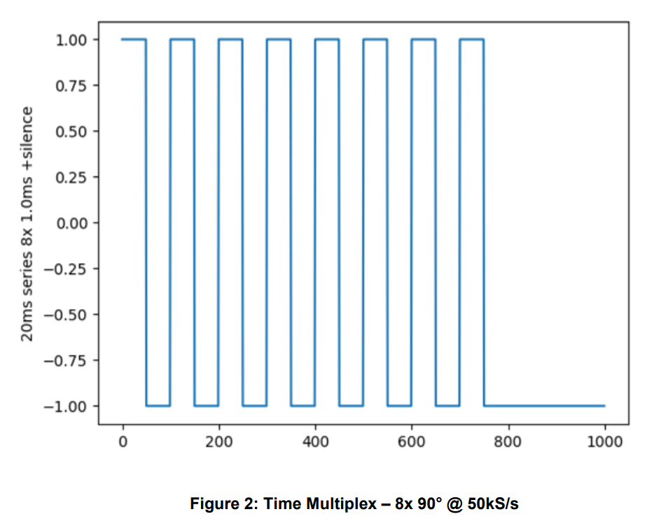
series=np.concatenate((pulse10, pulse10, pulse10, pulse10, pulse10, pulse10, pulse10, pulse10, si- lence), axis=None)
plt.plot(series)
plt.ylabel('20ms series 8x 1.0ms +silence')
plt.show()
second10=repeat48x(series)
plt.plot(second10)
plt.ylabel('1s- 20ms series 8x 1.0ms +silence')
plt.show()
#second1L
series=np.concatenate((pulse05, pulse10, pulse10, pulse10, pulse10, pulse10, pulse10, pulse10, si- lence), axis=None)
plt.plot(series)
plt.ylabel('1L- 20ms series 8x 1.0ms +silence')
plt.show()
second1L=repeat48x(series)
plt.plot(second1L)
plt.ylabel('1L-1s- 20ms series 8x 1.0ms +silence')
plt.show()
#second2L
series=np.concatenate((pulse10, pulse05, pulse10, pulse10, pulse10, pulse10, pulse10, pulse10, si- lence), axis=None)
plt.plot(series)
plt.ylabel('2L- 20ms series 8x 1.0ms +silence')
plt.show()
second2L=repeat48x(series)
plt.plot(second2L)
plt.ylabel('2L-1s- 20ms series 8x 1.0ms +silence')
plt.show()
#second3L
series=np.concatenate((pulse10, pulse10, pulse05, pulse10, pulse10, pulse10, pulse10, pulse10, si- lence), axis=None)
plt.plot(series)
plt.ylabel('3L- 20ms series 8x 1.0ms +silence')
plt.show()
second3L=repeat48x(series)
plt.plot(second3L)
plt.ylabel('3L-1s- 20ms series 8x 1.0ms +silence')
plt.show()
#second4L
series=np.concatenate((pulse10, pulse10, pulse10, pulse05, pulse10, pulse10, pulse10, pulse10, si- lence), axis=None)
plt.plot(series)
plt.ylabel('4L- 20ms series 8x 1.0ms +silence')
plt.show()
second4L=repeat48x(series)
plt.plot(second4L)
plt.ylabel('4L-1s- 20ms series 8x 1.0ms +silence')
plt.show()
#second5L
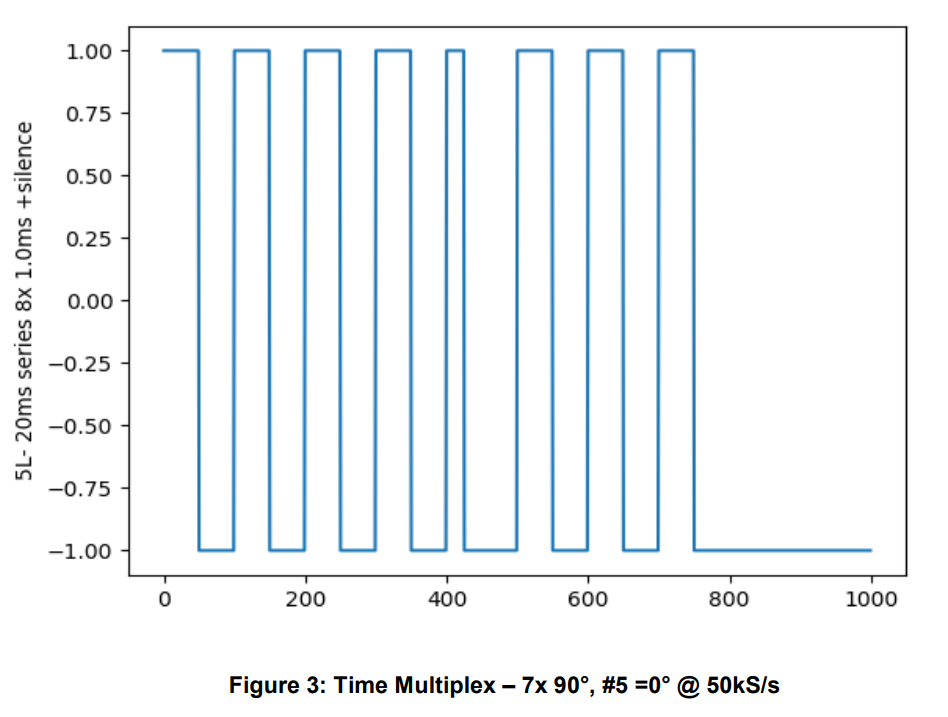
series=np.concatenate((pulse10, pulse10, pulse10, pulse10, pulse05, pulse10, pulse10, pulse10, si- lence), axis=None)
plt.plot(series)
plt.ylabel('5L- 20ms series 8x 1.0ms +silence')
plt.show()
second5L=repeat48x(series)
plt.plot(second5L)
plt.ylabel('5L-1s- 20ms series 8x 1.0ms +silence')
plt.show()
#second6L
series=np.concatenate((pulse10, pulse10, pulse10, pulse10, pulse10, pulse05, pulse10, pulse10, si- lence), axis=None)
plt.plot(series)
plt.ylabel('6L- 20ms series 8x 1.0ms +silence')
plt.show()
second6L=repeat48x(series)
plt.plot(second6L)
plt.ylabel('6L-1s- 20ms series 8x 1.0ms +silence')
plt.show()
#second7L
series=np.concatenate((pulse10, pulse10, pulse10, pulse10, pulse10, pulse10, pulse05, pulse10, silence), axis=None)
plt.plot(series)
plt.ylabel('7L- 20ms series 8x 1.0ms +silence')
plt.show()
second7L=repeat48x(series)
plt.plot(second7L)
plt.ylabel('7L-1s- 20ms series 8x 1.0ms +silence')
plt.show()
#second8L
series=np.concatenate((pulse10, pulse10, pulse10, pulse10, pulse10, pulse10, pulse10, pulse05, silence), axis=None)
plt.plot(series)
plt.ylabel('8L- 20ms series 8x 1.0ms +silence')
plt.show()
second8L=repeat48x(series)
plt.plot(second8L)
plt.ylabel('8L-1s- 20ms series 8x 1.0ms +silence')
plt.show()
w=wave.open("servo.wav", 'wb')
w.setnchannels(1)
w.setsampwidth(1)
w.setframerate(48000)
#w.setnframes(24000)
#w.setcomptype('NONE', 'wav')
w.writeframesraw(100*second10.astype(np.int8))
w.writeframesraw(100*second10.astype(np.int8))
w.writeframesraw(100*second10.astype(np.int8))
w.writeframesraw(100*second10.astype(np.int8))
w.writeframesraw(100*second1L.astype(np.int8))
w.writeframesraw(100*second2L.astype(np.int8))
w.writeframesraw(100*second3L.astype(np.int8))
w.writeframesraw(100*second4L.astype(np.int8))
w.writeframesraw(100*second5L.astype(np.int8))
w.writeframesraw(100*second6L.astype(np.int8))
w.writeframesraw(100*second7L.astype(np.int8))
w.writeframesraw(100*second8L.astype(np.int8))
w.writeframesraw(100*second10.astype(np.int8))
w.writeframesraw(100*second10.astype(np.int8))
w.writeframesraw(100*second10.astype(np.int8))
w.writeframesraw(100*second10.astype(np.int8))
w.close()
#servoMUX.py#####################################################################END#