Build a Smart Power Meter That Learns Your Appliances with NXP FRDM-IMX & ML

Using a hybrid machine learning model running on the powerful NXP FRDM-IMX93 board, our system can spot when a new appliance shows up and flag it for future identification. It's the perfect project to dive into the world of edge computing, IoT, and applied machine learning.

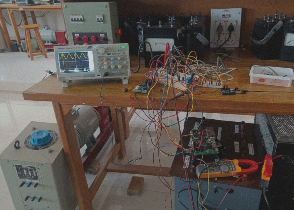
Our final hardware setup with sensors, the NXP board, and a resistive test load.

The Core Idea: A Two-Part Brain 

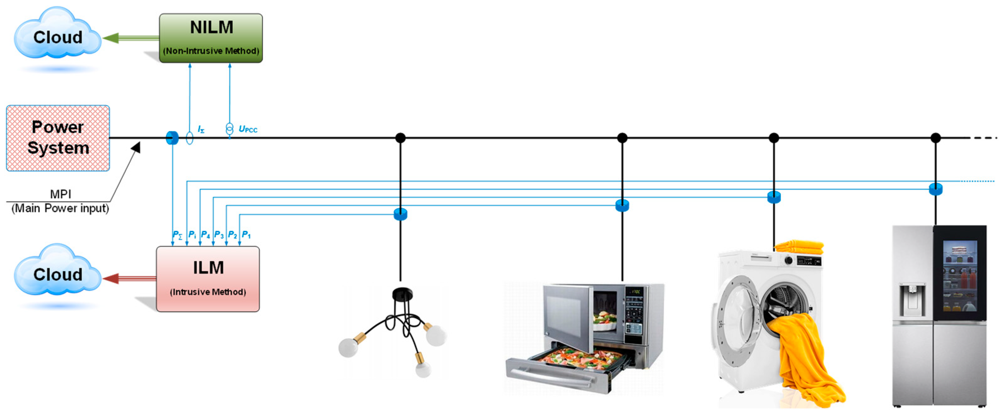
Our system's intelligence is split into two parts, working together to provide a complete picture of your home's energy use:

1. The Expert (Supervised Learning): First, we train a Random Forest model, which acts like an expert decision-maker. We show it the electrical signatures of known appliances (your fridge, microwave, fan, etc.) and it learns to recognize them instantly. When it sees a familiar pattern in the power data, it says, "Ah, that's the microwave turning on!"
2. The Watchdog (Unsupervised Learning): But what about new appliances? That's where our "watchdog" comes in. We use a mathematical tool called Jensen-Shannon (JS) Divergence to constantly monitor the "vibe" of your home's power stream. When the overall electrical signature suddenly changes in a way the "Expert" doesn't recognize, the JS Divergence score spikes. If it crosses a set threshold, the watchdog barks: "Hey, something new is happening here! A new appliance might be active."

This hybrid approach gives us the best of both worlds: the accuracy of a trained expert and the adaptability of a vigilant watchdog.

What You'll Need

Hardware:

• Main Controller: NXP FRDM-IMX93 evaluation board
• Voltage Sensor: ZMPT101B module (Safely measures mains voltage)
• Current Sensor: WCS1700 Hall-effect sensor (Safely and non-intrusively measures current)
• An external I2C ADC like the ADS1115 for high-resolution readings.
• Extension board, resistive load (for testing), and jumper wires.

Software & Libraries:

• Python: For data analysis and machine learning (Pandas, Scikit-learn, NumPy).
• NXP MCUXpresso IDE: For programming the Cortex-M33 core.
• Embedded Linux (Yocto): For the Cortex-A55 core.
• C/C++: For the real-time firmware on the M33.

Step 1: Safe Sensing (The Hardware)

The most critical part is measuring mains electricity safely.

• The ZMPT101B sensor connects in parallel with the main line. It uses a transformer to provide galvanic isolation, protecting our low-voltage electronics.
• The WCS1700 current sensor is even safer; the main wire simply loops through it. It measures the magnetic field to determine current, meaning it's completely electrically isolated.
• Connect the analog outputs of these sensors to an I2C ADC (like the ADS1115), which is then wired to the FRDM-IMX93's LPI2C pins.

Step 2: High-Fidelity Data Capture (Cortex-M33's Job)

On the M33 core, we run a simple firmware written in C/C++ using the MCUXpresso IDE.

• Its only job is to continuously read data from the I2C ADC at a fixed frequency (e.g., 3.2 kHz).
• It collects the data into a buffer (e.g., 500 samples).
• Once the buffer is full, it sends it over to the A55 core using the Remote Processor Messaging (RPMsg) framework, which is designed for this kind of inter-core communication.

Step 3: Feature Engineering in Linux (Cortex-A55's Job)

A Python script running on the A55's Linux OS receives the raw waveform data. It then:

1. Calculates Features: It computes the true RMS Voltage, RMS Current, Real Power, and Power Factor from the raw samples.
2. Creates a Feature Vector: It bundles the three most important features we identified—Voltage, Current, and Power Factor—into a simple array. This vector is now ready to be fed to our models.

PCA shows how different appliances form distinct clusters using just a few electrical features.

Step 4: On-Device Intelligence (The ML Models)

Finally, the Python script uses the feature vector to perform the two-part analysis:

1. Random Forest Inference: It feeds the vector to our pre-trained Random Forest model using Scikit-learn. The model returns its prediction for which known appliance is active.
2. JS Divergence Calculation: The script compares the statistical distribution of the latest batch of feature vectors to a historical baseline. A spike in the JS Divergence score means a "concept drift" has occurred, and it triggers a "New Appliance Detected!" alert.

When a new appliance turns on, the JS Divergence (blue) spikes above the threshold (red), signaling an event.

Step 1: Safe Sensing (The Hardware)

The most critical part is measuring mains electricity safely.

• The ZMPT101B sensor connects in parallel with the main line. It uses a transformer to provide galvanic isolation, protecting our low-voltage electronics.
• The WCS1700 current sensor is even safer; the main wire simply loops through it. It measures the magnetic field to determine current, meaning it's completely electrically isolated.
• Connect the analog outputs of these sensors to an I2C ADC (like the ADS1115), which is then wired to the FRDM-IMX93's LPI2C pins.

Step 2: High-Fidelity Data Capture (Cortex-M33's Job)

On the M33 core, we run a simple firmware written in C/C++ using the MCUXpresso IDE.

• Its only job is to continuously read data from the I2C ADC at a fixed frequency (e.g., 3.2 kHz).
• It collects the data into a buffer (e.g., 500 samples).
• Once the buffer is full, it sends it over to the A55 core using the Remote Processor Messaging (RPMsg) framework, which is designed for this kind of inter-core communication.

Step 3: Feature Engineering in Linux (Cortex-A55's Job)

A Python script running on the A55's Linux OS receives the raw waveform data. It then:

1. Calculates Features: It computes the true RMS Voltage, RMS Current, Real Power, and Power Factor from the raw samples.
2. Creates a Feature Vector: It bundles the three most important features we identified—Voltage, Current, and Power Factor—into a simple array. This vector is now ready to be fed to our models.

PCA shows how different appliances form distinct clusters using just a few electrical features.

Step 4: On-Device Intelligence (The ML Models)

Finally, the Python script uses the feature vector to perform the two-part analysis:

1. Random Forest Inference: It feeds the vector to our pre-trained Random Forest model using Scikit-learn. The model returns its prediction for which known appliance is active.
2. JS Divergence Calculation: The script compares the statistical distribution of the latest batch of feature vectors to a historical baseline. A spike in the JS Divergence score means a "concept drift" has occurred, and it triggers a "New Appliance Detected!" alert.

When a new appliance turns on, the JS Divergence (blue) spikes above the threshold (red), signaling an event.

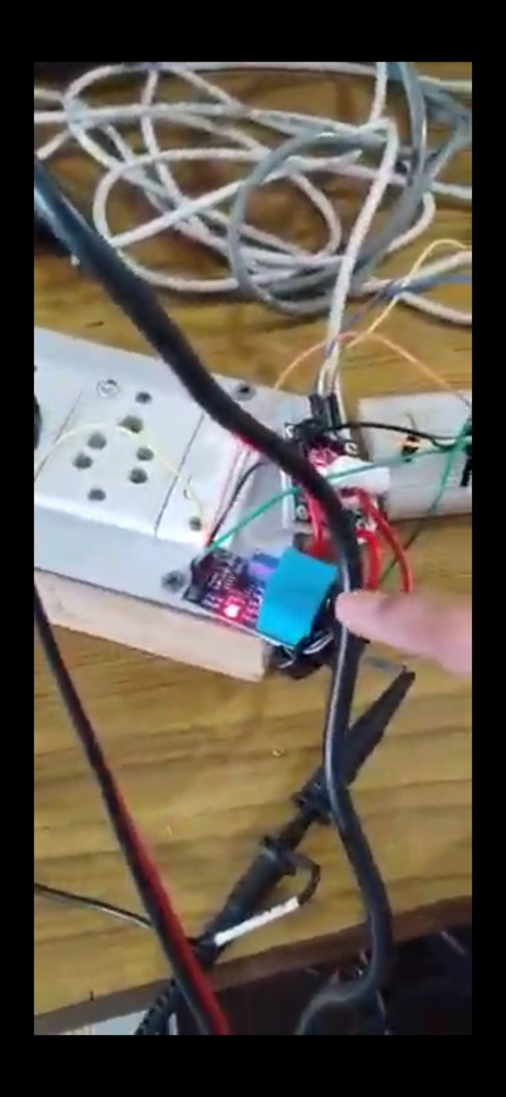
Final Hardware Setup:

● The main supply was connected to an extension board.

● The ZMPT101B voltage sensor was connected across the extension board output to

measure line voltage.

● The Hall Effect–based current sensor was connected looped around the wiring to sense

current safely.

● Both sensors’ outputs were connected to the appropriate analog pins of the Arduino.

● A single phase resistive load (comprising multiple switchable knobs) was connected as the

primary load to the extension board.

● An oscilloscope was used to verify the voltage waveforms captured by the ZMPT sensor.

● A power analyzer measured real-time power, power factor, and voltage, serving as a

ground truth reference.

● A clamp meter was used to independently measure the current through the load for

cross-verification.

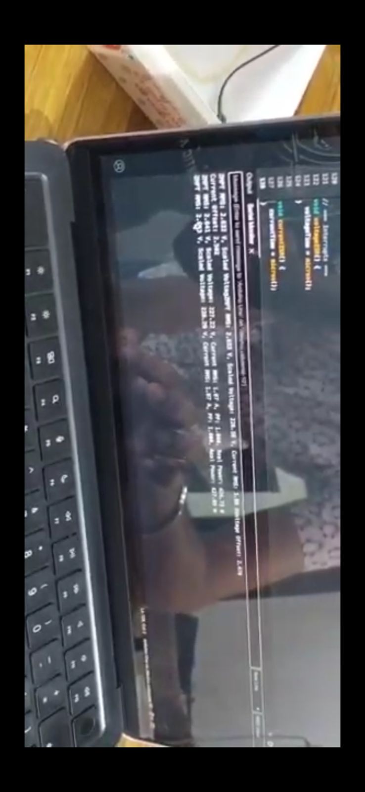
The Arduino was programmed to read the analog voltages, apply the necessary scaling and

calibration offsets, and compute the real-time voltage, current, power, and power factor. These

computed values were displayed continuously, providing live feedback.

Calibration was performed by adjusting offset values to match the Arduino’s measured parameters

with the readings from the power analyzer and clamp meter.

We validated the setup by switching on and off different knobs of the resistive load bank and

observing the corresponding changes in real-time measurements. The data was sent through I2c to the NXP board.

The system responded accurately, demonstrating negligible errors across a wide range of load

conditions.

Thus, the final hardware system ensured both safety (through isolation) and accuracy (through

proper sensor selection and calibration), enabling reliable real-time data collection for NILM

experimentation. The hardware setup looked as -

Challenges, Scalability, and the Path to a Universal Solution

Building a prototype that works in a controlled lab environment is one thing; creating a device that works reliably in any home is another. Here are some of the key challenges we faced and how this system can be evolved into a more robust, universally applicable solution.

Problems Faced & Real-World Hurdles

1. The Multiple Appliance Problem: What happens when you turn on the microwave while the fridge compressor is already running? Their electrical signatures overlap, creating a new, combined signature that can easily confuse a simple model. Our system might flag this as a "new appliance" rather than identifying the two separate devices.
2. "Noisy" Power Lines: Many modern devices, especially those with motors (blenders, fans) or switching power supplies (laptops, TVs), introduce high-frequency noise and harmonics onto the power line. This "noise" can distort the clean sine wave we expect to see, making it harder to calculate accurate features and identify appliances.
3. Similar-Signature Appliances: Two different brands of incandescent light bulbs or two similar-sized resistive heaters can have nearly identical power signatures in their steady state. Distinguishing between them using only basic features like V, A, and PF is extremely difficult.

Making a Better, More Scalable Solution

To overcome these challenges and build a truly "smart" meter, we need to upgrade our approach. The NXP FRDM-IMX93 is perfectly equipped for these next steps.

1. The Power of Transients: The most unique part of an appliance's signature is the transient—the sharp, complex electrical spike that occurs in the first few milliseconds after it's switched on. This transient is like a fingerprint, packed with high-frequency details that are unique even for appliances that seem identical in their steady state.

• How to Implement It:
• Increase the sampling rate on the Cortex-M33 core significantly to capture these ultra-fast events.
• Program the M33 to detect a sudden change in current, capture a high-resolution snapshot of the transient, and send that specific data to the A55 core for analysis.

2. Graduating to a Neural Network on the NPU: While Random Forest is great, it's not the best tool for analyzing complex waveforms like transients. For this, we need to move to a 1D Convolutional Neural Network (CNN).

• Why a CNN? CNNs are brilliant at finding patterns in sequential data. We can train a 1D CNN to look directly at the raw transient waveform and learn to identify the subtle patterns that differentiate a blender motor from a vacuum cleaner motor.
• Leveraging the NPU: This is where the FRDM-IMX93 truly shines. Using NXP's eIq Toolkit, we can train a lightweight CNN and deploy it to the onboard Neutron NPU. This offloads the entire complex inference task, allowing it to run incredibly fast and efficiently without bogging down the main Cortex-A55 processor.

This NPU-accelerated CNN approach is the key to solving the multiple appliance and similar-signature problems, making the system far more accurate and scalable.

Conclusion

This project demonstrates that by intelligently combining supervised and unsupervised machine learning on a powerful multi-core edge device like the NXP FRDM-IMX93, we can create a truly smart and adaptable power meter. We've successfully built a system that not only identifies known devices but also learns to recognize when new ones appear.

While real-world challenges exist, the path forward is clear. By leveraging advanced techniques like transient analysis and accelerating neural networks on the onboard NPU, this platform has the potential to become a highly accurate, universally applicable energy monitoring solution. This project is more than just a smart meter; it's a window into the future of edge AI, where intelligent devices can help us better understand and manage our world.